- Authors:
- W.G.C.W. Kumara (
chinthakawk@gmail.com) - Timothy K. Shih (
timothykshih@gmail.com)
Introduction
This paper presents research findings on calibrating RGB-D information from an array of RGB-D sensors to construct a 3D model of a human bust and a puppet. RGB-D information of each RGB-D sensor are first collected at a centralized PC and point clouds are generated. Point clouds are aligned using a color-based duplicate removal iterative closest point algorithm. Two noise removal algorithms are introduced before and after the alignment to remove the outliers. A 8-neighbor 3D super-resolution algorithm is introduced to increase the point cloud quality. Next, small hole filling mechanisms and large hole filling in 3D based on 2D inpainting are proposed. Finally, a 3D Poisson surface is created. Main contributions of this work are, color-based duplicate removal iterative closest point algorithm, noise removal, super- resolution, and 3D inpainting based on 2D inpainting. Experimental results demonstrate that the proposed strategic steps provide a better 3D model.
Keywords
3d reconstruction, kinect, icp, noise removal, inpainting, hole filling
Proposed Method
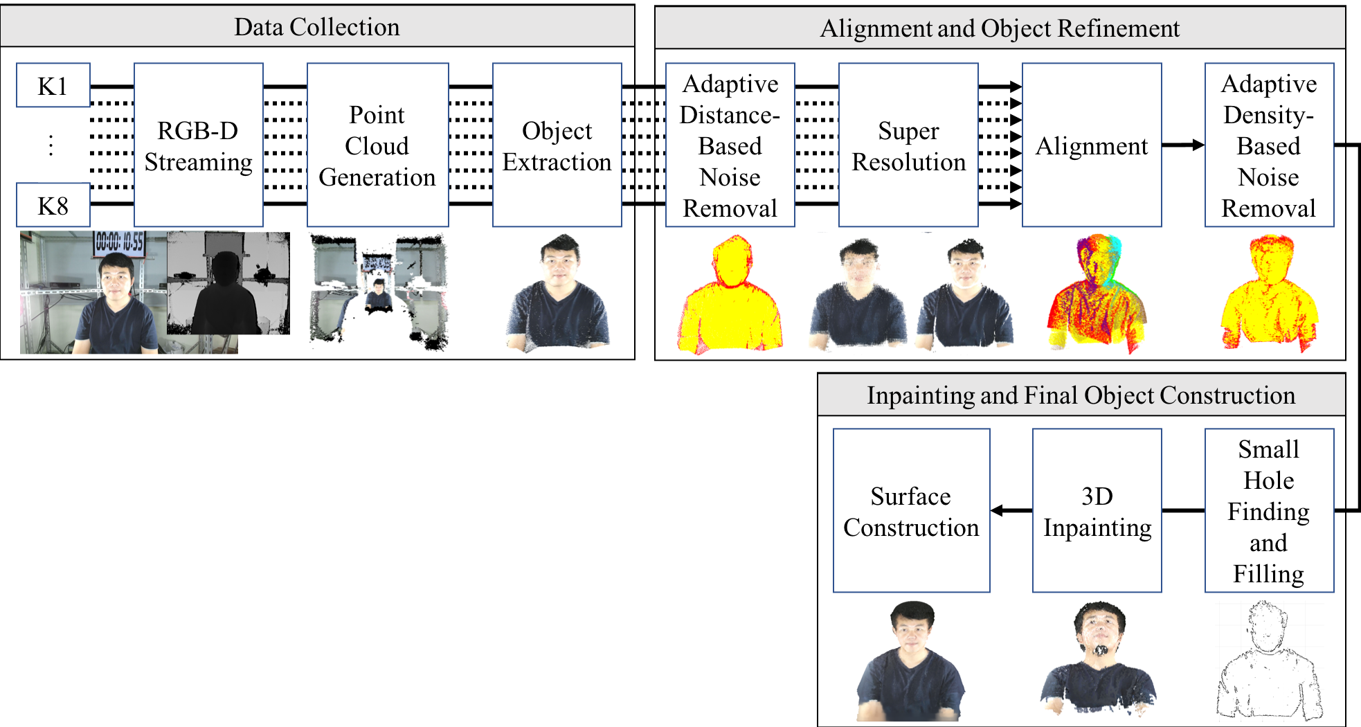
Data Collection
RGB-D sensors can be used to capture color and depth images of the scene. We first project the depth pixel values in to the color image space. Then depth values are projected in to the camera space or the 3D space. Next, we can copy the corresponding color values from the color image to the point cloud. The result is a colored 3D point cloud. As we focus only on 3D reconstruction of the objects or human bust here, we first need to extract only the object from the complete point cloud. A predefined depth threshold is used to extract the object.
Alignment and Object Refinement
Noise removal of the point clouds
RGB-D sensor depth image values are not always correct. Depth image may contain noise due to several factors such as inherent camera problems, projection issues, interferences from the surrounding, interferences from the other sensors, etc. We need to remove noise points from the point clouds before proceeding. Two noise removal algorithms are proposed here in order to obtain a noise free point cloud. Noise points are dense around the edges of the objects and the density is proportional to the distance from the sensor. Hence, the first noise removal algorithm removes noise points from each point cloud created from each sensor. This is called adaptive distance-based noise removal algorithm. Next noise removal is performed after align point clouds from all sensors. After align all the point clouds, points are independent from the original sensor. Hence the second algorithm is called adaptive density- based noise removal algorithm and performed after the merging of point clouds.

8-neighbor 3D super-resolution
After the noise removal of the point cloud, a 3D super-resolution method is applied on the point cloud to increase the number of points. Newly introduced points in the super-resolution step helps filling small holes in the point cloud. Color and depth image resolutions of the RGB-D sensor are different. Point cloud is generated from the depth image and only the corresponding color values are copied. Since the color image resolution is higher comparing to the depth image, by bringing in some extra points from the color image as new points to the point cloud, number of points in the point cloud can be easily increased.

Point cloud alignment with color-based duplicate-removal ICP
Point coordinates of a point in a surface captured from two RGB-D sensors at two locations are different as the two sensors use individual coordinate systems. In order to construct a 3D object from the multiple point clouds, first, point clouds must be aligned correctly. Iterative closest point (ICP) algorithm is used to align two point clouds. ICP works if the two point clouds are in a close proximity. Since a sensor pair is around 45◦ apart in our setup, first two clouds are required to be brought to a coarse alignment. We placed a paper with four different color rectangle markers in the middle of the set up and recorded once from all the sensors. Then the user marks three corresponding point pairs in both color views (Figure 4(a)). We require at least three point pairs to find transformation matrix in Euclidian space. Red points marked are the points with available depth values from the depth im- age. The corresponding 3D coordinates for the user marked points are found from the point clouds. Found 3D coordinates from two clouds are used to find the transformation matrix of the rough alignment phase using the single value decomposition. In 4(b), red circles are user marked 3 points in the reference point cloud (pcr) A, green circles are user marked 3 correspoinding points in the source point cloud (pcs) (B), and blue crosses are coarse aligned corresponding source points (B2). Then, ICP is used to find a fine alignment considering of the coarse aligned point clouds.

Inpainting and Final Object Construction
There may be large holes available in the point cloud due to occlusion as the chin hole in Figure 6(a). The proposed large hole filling consists of two steps as finding large holes and filling large holes. The purpose is to fill holes on a 3D model using 2D image inpainting.

Experimental Results
Setup
We used two setups during the experiment. In the first setup, 8 RGB- D sensors were placed 1m height at 45◦ angles in the circumference of a 1.5m diameter circle to record a person sitting in the center of the circle as in Figure 8.

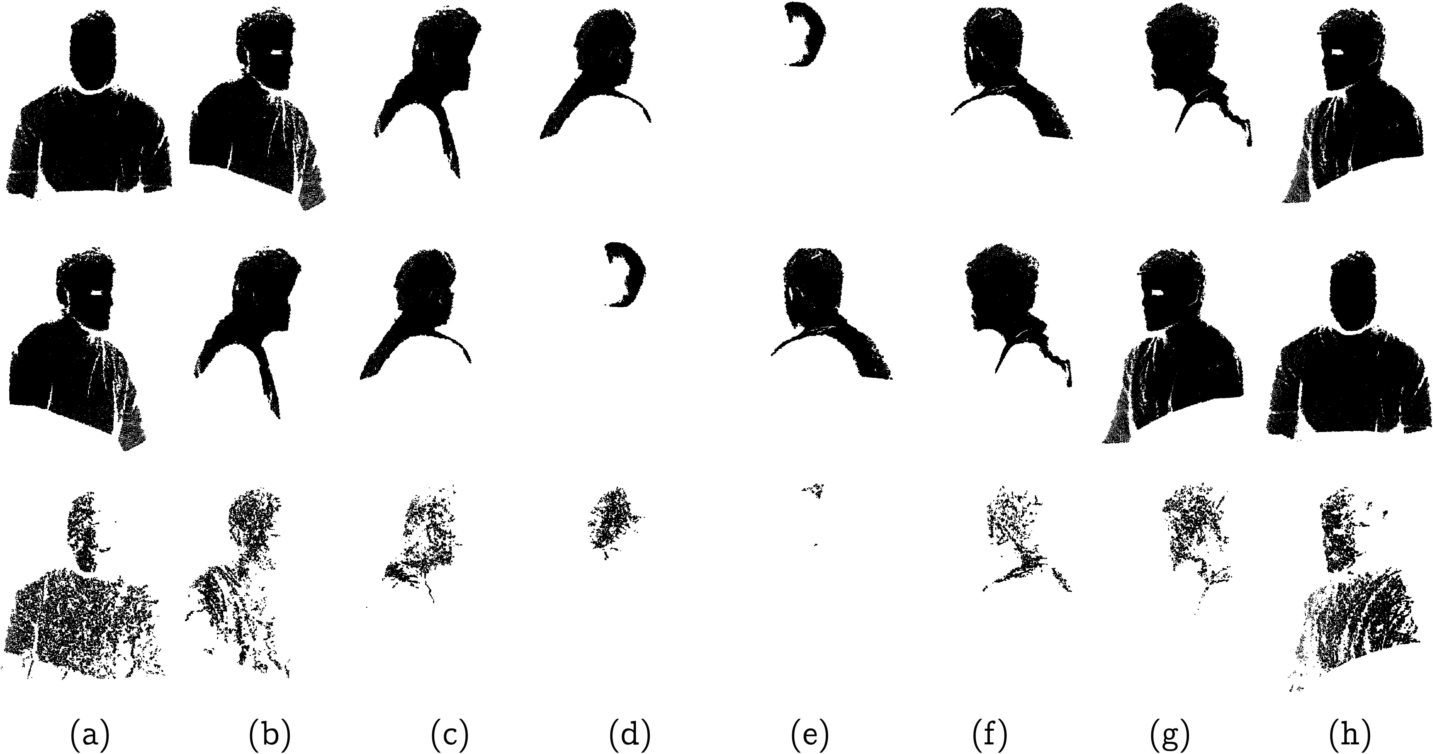
Adaptive distance-based noise removal
Person bust was then separated from the original point clouds of the synchronized frames using distance thresholds along x, y, and z axes. Next, adaptive distance-based noise removal performed to remove noise points in each point cloud. The effect of different outlier probability op values are shown in Table 2. For the rest of the examples op = 0.15 was used.


8-neighbor 3D super-resolution

Small hole finding


 |
Results: Setup 1


Results: Setup 2

SIM and MSE
Surface Interpenetration Measure (SIM), Mean Squared Error (MSE)

 |
 |

 |

 |
References
- W. G. C. W. Kumara, S.-H. Yen, H.-H. Hsu, T. K. Shih, W.-C. Chang, E. Togootogtokh, Real-time 3d human objects rendering based on mul- tiple camera details, Multimedia Tools and Applications 76 (9) (2017) 11687–11713.
- B. Bellekens, V. Spruyt, R. Berkvens, R. Penne, W. M., A benchmark survey of rigid 3d point cloud registration algorithms, International Journal on Advances in Intelligent Systems 8 (12) (2015) 118–127.
- G. Elbaz, T. Avraham, A. Fischer, 3d point cloud registration for local- ization using a deep neural network auto-encoder, in: 2017 IEEE Con- ference on Computer Vision and Pattern Recognition (CVPR), IEEE, 2017, pp. 2472–2481.
- S. Rusinkiewicz, M. Levoy, Efficient variants of the icp algorithm, in: Proceedings of the Third International Conference on 3-D Digital Imag- ing and Modeling, IEEE, 2001, pp. 145–152.
- S. Bouaziz, A. Tagliasacchi, M. Pauly, Sparse iterative closest point, in: Computer graphics forum, Vol. 32, Wiley Online Library, 2013, pp. 113–123.
- J. Yang, H. Li, Y. Jia, Go-icp: Solving 3d registration efficiently and globally optimally, in: Proceedings of the IEEE International Conference on Computer Vision, 2013, pp. 1457–1464.
- M. Keller, D. Lefloch, M. Lambers, S. Izadi, T. Weyrich, A. Kolb, Real- time 3d reconstruction in dynamic scenes using point-based fusion, in: International Conference on 3D Vision, IEEE, 2013, pp. 1–8.
- D. Gallup, J.-M. Frahm, P. Mordohai, Q. Yang, M. Pollefeys, Real- time plane-sweeping stereo with multiple sweeping directions, in: IEEE Conference on Computer Vision and Pattern Recognition, IEEE, 2007, pp. 1–8.
- X. Zabulis, K. Daniilidis, Multi-camera reconstruction based on surface normal estimation and best viewpoint selection, in: Proceedings of the 2nd International Symposium on 3D Data Processing, Visualization and Transmission, IEEE, 2004, pp. 733–740.
- Y. Furukawa, J. Ponce, Accurate, dense, and robust multiview stereopsis, IEEE transactions on pattern analysis and machine intelligence 32 (8) (2010) 1362–1376.
- C. E. Scheidegger, S. Fleishman, C. T. Silva, Triangulating point set surfaces with bounded error., in: Symposium on Geometry Processing, 2005, pp. 63–72.
- Y. Liu, Q. Dai, W. Xu, A point-cloud-based multiview stereo algorithm for free-viewpoint video, IEEE transactions on visualization and com- puter graphics 16 (3) (2010) 407–418.
- Y. Alj, G. Boisson, P. Bordes, M. Pressigout, L. Morin, Space carving mvd sequences for modeling natural 3d scenes, in: Three-Dimensional Image Processing (3DIP) and Applications II, 2012, pp. 1–8.
- W. E. Lorensen, H. E. Cline, Marching cubes: A high resolution 3d surface construction algorithm, in: ACM siggraph computer graphics, Vol. 21, ACM, 1987, pp. 163–169.
- S. M. Seitz, C. R. Dyer, Photorealistic scene reconstruction by voxel coloring, in: Proceedings of the IEEE Computer Society Conference on Computer Vision and Pattern Recognition, IEEE, 1997, pp. 1067–1073.
- K. N. Kutulakos, S. M. Seitz, A theory of shape by space carving, in: The Proceedings of the Seventh IEEE International Conference on Computer Vision, Vol. 1, IEEE, 1999, pp. 307–314.
- K. Kutulakos, Approximate n-view stereo, European Conference on Computer Vision (2000) 67–83.
- C. H. Esteban, F. Schmitt, Silhouette and stereo fusion for 3d object modeling, Computer Vision and Image Understanding 96 (3) (2004) 367–392.
- M. Goesele, B. Curless, S. M. Seitz, Multi-view stereo revisited, in: IEEE Computer Society Conference on Computer Vision and Pattern Recognition, Vol. 2, IEEE, 2006, pp. 2402–2409.
- J. Park, H. Kim, Y.-W. Tai, M. S. Brown, I. Kweon, High quality depth map upsampling for 3d-tof cameras, in: IEEE International Conference on Computer Vision, IEEE, 2011, pp. 1623–1630.
- J. Becker, C. Stewart, R. J. Radke, Lidar inpainting from a single im- age, in: 12th International Conference on Computer Vision Workshops, IEEE, 2009, pp. 1441–1448.
- C. Zhang, Q. Cai, P. A. Chou, Z. Zhang, R. Martin-Brualla, Viewport: A distributed, immersive teleconferencing system with infrared dot pat- tern, IEEE MultiMedia 20 (1) (2013) 17–27.
- A. Smolic, 3d video and free viewpoint videofrom capture to display, Pattern recognition 44 (9) (2011) 1958–1968.
- G. H. Bendels, R. Schnabel, R. Klein, Detecting holes in point set sur- faces, The Journal of WSCG 14 (2006) 89–96.
- A. Telea, An image inpainting technique based on the fast marching method, Journal of graphics tools 9 (1) (2004) 23–34.
- A. Criminisi, P. P ́erez, K. Toyama, Region filling and object removal by exemplar-based image inpainting, IEEE Transactions on image process- ing 13 (9) (2004) 1200–1212.
- M. Kazhdan, H. Hoppe, Screened poisson surface reconstruction, ACM Transactions on Graphics (TOG) 32 (3) (2013) 29.
- L. Silva, O. R. P. Bellon, K. L. Boyer, Precision range image registration using a robust surface interpenetration measure and enhanced genetic algorithms, IEEE transactions on pattern analysis and machine intelli- gence 27 (5) (2005) 762–776.
Contact Us
For any questions or comments regarding this content please contact:
Timothy K. Shih (timothykshih@gmail.com).

Timothy K. Shih is a Distinguished Professor at the National Central University, Taiwan. He was the Dean of the College of Computer Science, Asia University, Taiwan and the Chairman of the CSIE Department at Tamkang University, Taiwan. Prof. Shih is a Fellow of the Institution of Engineering and Technology (IET). He was also the founding Chairman Emeritus of the IET Taipei Local Network. In addition, he is a senior member of ACM and a senior member of IEEE. Prof. Shih joined the Educational Activities Board of the IEEE Computer Society. He was the founder and co-editor-in-chief of the International Journal of Distance Education Technologies, USA. He is the Associate Editor of IEEE Computing Now. And, he was the associate editors of the IEEE Transactions on Learning Technologies, the ACM Transactions on Internet Technology, and the IEEE Transactions on Multimedia. Prof. Shih was the Conference Co-Chair of the 2004 IEEE International Conference on Multimedia and Expo (ICME'2004). He has been invited to give more than 50 keynote speeches and plenary talks in international conferences, as well as tutorials in IEEE ICME 2001 and 2006, and ACM Multimedia 2002 and 2007. Prof. Shih's current research interests include Multimedia Computing, Computer-Human-Interaction, and Distance Learning. He has edited many books and published over 500 papers and book chap- ters. Prof. Shih has received many research awards, including research awards from National Science Council of Taiwan, IIAS research award from Germany, HSSS award from Greece, Brandon Hall award from USA, the 2015 Google MOOC Focused Research Award, and sev- eral best paper awards from international conferences. Professor Shih was named the 2014 Outstanding Alumnus by Santa Clara University. http://www.csie.ncu.edu.tw/tshih
http://tshih.minelab.tw/tshih